As someone who loves playing around with data, I recently took on a project to analyse the Adult Income dataset using Pandas —a powerful Python library for data manipulation and analysis.
If you’re wondering what that means, I’m here to walk you through everything step by step. If you’re new to data or just curious, Don’t worry; I’ve got you covered.
Allow me to take you through it!
First, have you ever heard the term EDA? If you’re thinking, “Is that some sort of secret code?” — don’t worry, you’re not alone 😄! It stands for Exploratory Data Analysis, but it’s not as complicated as it sounds.
Exploratory Data Analysis, or EDA for short, investigates a dataset to discover patterns and anomalies (outliers) and form hypotheses based on our understanding.
It’s basically like giving your data a good once-over. You clean it up, check it out from different angles, and see what interesting things it has to say
EDA is super important because it helps you figure out what to do next with your dataset: maybe build a cool machine learning model, or if the data is too messy, sometimes you must say goodbye and start fresh with new data!
1. Dataset Overview
So, what’s this dataset all about? Well, the Adult Income dataset is a collection of data about different people—things like their age, race, education, job, how much they earn, etc.
It’s a popular dataset in the Kaggle Team, and it’s perfect for exploring how different factors might influence income.
Before I could dive into the fun part (the analysis!), I had to do some housekeeping to get the data ready.
Think of it like tidying up your desk before starting a new project.
This meant checking for missing pieces and ensuring everything was in a format that Pandas could understand.
2. Getting to Know the Data
Now, let’s discuss the steps I took to familiarize myself with the data.
It’s like getting to know a new friend or going on a date—you ask a few questions, check out some details, and you’re on the same page before you know it.
So, to learn what this dataset implies, I imported the dataset.
Importing the Data
We first need to bring the data into our workspace to start our journey. Here’s how I did it: I told Python I wanted to use Pandas for fast analysis, data cleaning, and preparation.
RELATED: How AI Learns and Adapts: The Technology Behind Smarter Apps
Then, I gave it the nickname. pd So it’s easier to use. Then, I imported Matplotlib to create static, animated, and interactive visualizations. Lastly, I imported Seaborn, a Python data visualization library based on Matplotlib.
It provides a high-level interface for drawing attractive and informative statistical graphics.
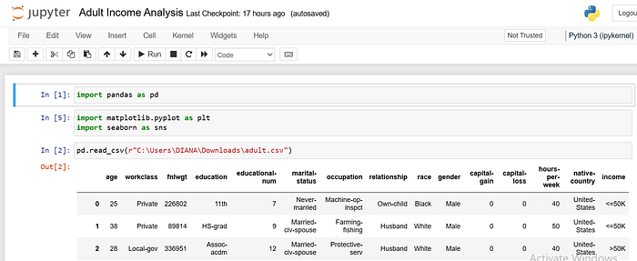
I used Pandas to load the dataset from a CSV file. The pd.read_csv() function helps us open up a big box of data and lay it out before the analysis.
We tell it where the file is located on our computer, and it loads all that data into a DataFrame, which we’ve named it.df.

head()
I asked Pandas to show me the first six rows of the data. To get a quick snapshot of what’s inside our data, The head() function helps us flip through the first few columns to see what’s inside.
Bypassing the number 6 into the function, we’re telling Pandas to show us the first six rows of the DataFrame.
This helps us quickly understand what the data looks like and what kinds of information it contains.

tail()
I asked Pandas to show me the last six rows of the data. To get a quick snapshot of what’s inside our data, The tail() function helps us flip through the last few columns to see what’s inside.
By passing the number 6 into the function, we’re telling Pandas to show us the last six rows of the DataFrame.

info()
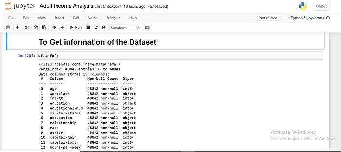
This function asks the DataFrame to introduce itself. It gives us a summary of the data, including the number of rows and columns, the types of data in each column (like numbers, text, etc.), and whether any values are missing.
It’s a quick way to understand the structure of the dataset and spot potential issues at first glance.
df.shape
Imagine figuring out a puzzle’s size before you start putting it together. The shape attribute tells us the dimensions of the DataFrame, specifically the number of rows and columns.
It returns a tuple like(rows, columns), so you can see at a glance how much data you’re working with.

Null Values
Null values represent missing or undefined data in your dataset. In the context of data analysis, a null value means no information is available for a particular entry in a specific column.
In Pandas, null values are typically represented as NaN, which stands for “Not a Number.”
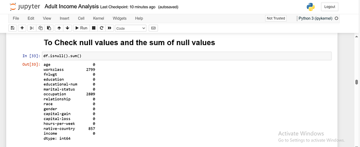
We can identify null values in a DataFrame using the isnull() function, which returns a DataFrame of the same shape as the original, but with True for every null entry and False otherwise.
You can also use sum() to get the total count of null values for each column.
Visualizing Null Values with Seaborn
sns.heatmap(df.isnull()): This line creates a heatmap where each cell in the DataFrame is coloured according to whether it is null (True or False).

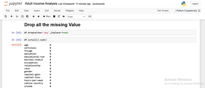
To Drop All Missing Values
Removing rows with missing data is sometimes better than trying to fill them in.
This might be the case if there are too many missing values or if the missing values are in a column that isn’t crucial to your analysis.
To drop columns, you can use the drop() function. You need to specify the column names and set axis=1 them to indicate that you’re dropping columns (not rows), inplace=True apply the changes directly to the original DataFrame.
Duplicate values
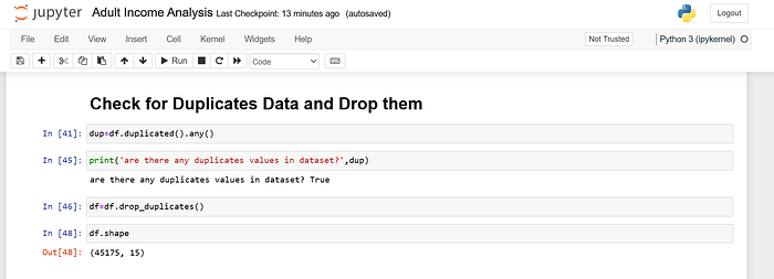
Duplicate values are entries in your dataset that appear more than once. For example, if the same person’s information appears twice in your dataset, that would be a duplicate.
Duplicates can distort your analysis by giving too much weight to certain data points.
For example, if the income data for a particular person appears twice, it could incorrectly influence the results of any analysis or calculations you perform.
Pandas make it easy to identify and remove duplicate rows. You can use the duplicated() function to see which rows are duplicates and the drop_duplicates() function to remove them.
Dropping Unnecessary Columns
Sometimes, removing rows with missing data is better than trying to fill them in. This might be the case if there are too many missing values or if the missing values are in a column that isn’t crucial to your analysis.
You can drop rows with missing values using the dropna() function. This function removes any row that contains at least one NaN value.
If you want to remove columns with missing values instead of rows, you can specify axis=1.

Final Thoughts
And there you have it! We’ve successfully imported, explored, and cleaned up the Adult Income dataset. Through these steps, I hope you understand what this dataset is all about and how different factors might influence a person’s income.
It’s been an exciting journey, and I can’t wait to dive deeper into the analysis!
If this sparked your curiosity and you want to see more, you can check out the full code and dataset on my GitHub. As always, feel free to reach out if you have any questions or just want to chat about data—I’m here for it 😊!

